Time Series Models

Time Series Example
The purpose of this bog is compare the performance of some forecast methods in order to select the best option.
Import packages and additional functions
library(dplyr)
library(readr)
library(forecast)
library(xts)

# functions
rmse <- function(real,prediction){
  error <- real - prediction
  return( sqrt(mean(error^2)) )
}

plot_df <- function(df, title_text){
  plot(xts( df[,c('real','prediction')], order.by = df$row ) ,
       type = "l", main = title_text, col = c("#ff3644","#2f002f"),
       ylab = 'values', legend.loc = "bottomleft", lty = c("solid","dashed") )
}

create_df_compare <- function(real, prediction){
  df <- data.frame(real= real ,prediction = prediction,
             row =  seq(as.Date('1987-03-01'), length = length(real), by = "month") )
  return(df)
}
Load data set
First, I loaded the .dat file and then plotted the time series to make a visual analysis.
variable <- round(read.delim('serie.dat',header=FALSE),2)
cat('The file has: ', nrow(variable), 'observations.\n')
## The file has: 168 observations.summary(variable)## V1
## Min. :20.00
## 1st Qu.:23.28
## Median :24.95
## Mean :25.06
## 3rd Qu.:26.88
## Max. :30.00plot(xts(x= variable$V1,
order.by = seq(as.Date('1976-01-01'), length = length(variable$V1), by = "month")),
type="l", col="#2f002f", lwd=2, main = 'Evolution of Time serie', ylab = 'Values')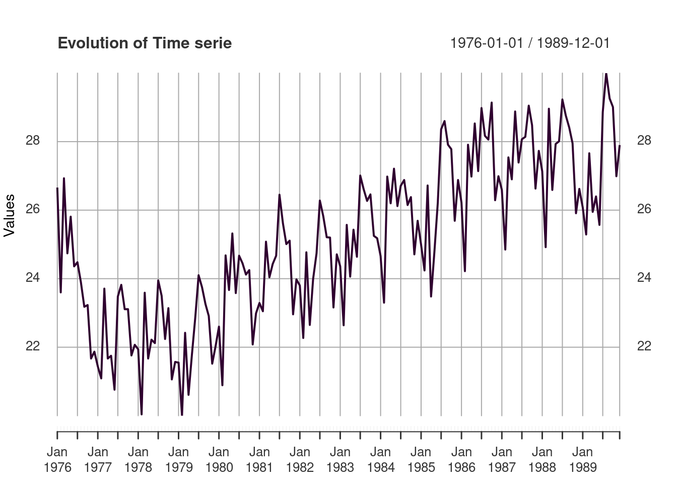
Split in train and test data set
Subsequently, I divided the total data in train (80%) and test (20%).
- The Train data had 134 observations (from “1976-01-01” to “1987-02-01”).
- The Train data had 34 observations (from “1987-02-01” to “1989-11-01”).
Also, I show the plots about train and test data.
train_df <- variable[1:round(length(variable$V1)*0.8,0), ]
test_df <- variable[(round(length(variable$V1)*0.8,0)+1): nrow(variable), ]

par(mfrow=c(2,1), mar=c(3,4,3,1))
plot(xts(x= train_df, order.by = seq(as.Date('1976-01-01'), length = length(train_df), by = "month") ) ,
     type="l", col="#2f002f", main ='time series variable- train')
plot(xts(x= test_df, order.by = seq(as.Date('1987-02-01'), length = length(test_df), by = "month")),
     type="l", col="#2f002f", main ='time series variable-test')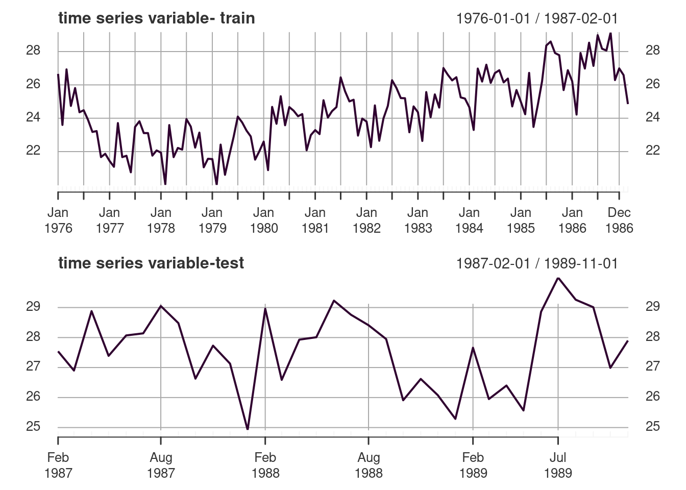
Time serie Descomposition
descomp <- decompose(ts(train_df,frequency = 12,start = 1976))
plot(descomp)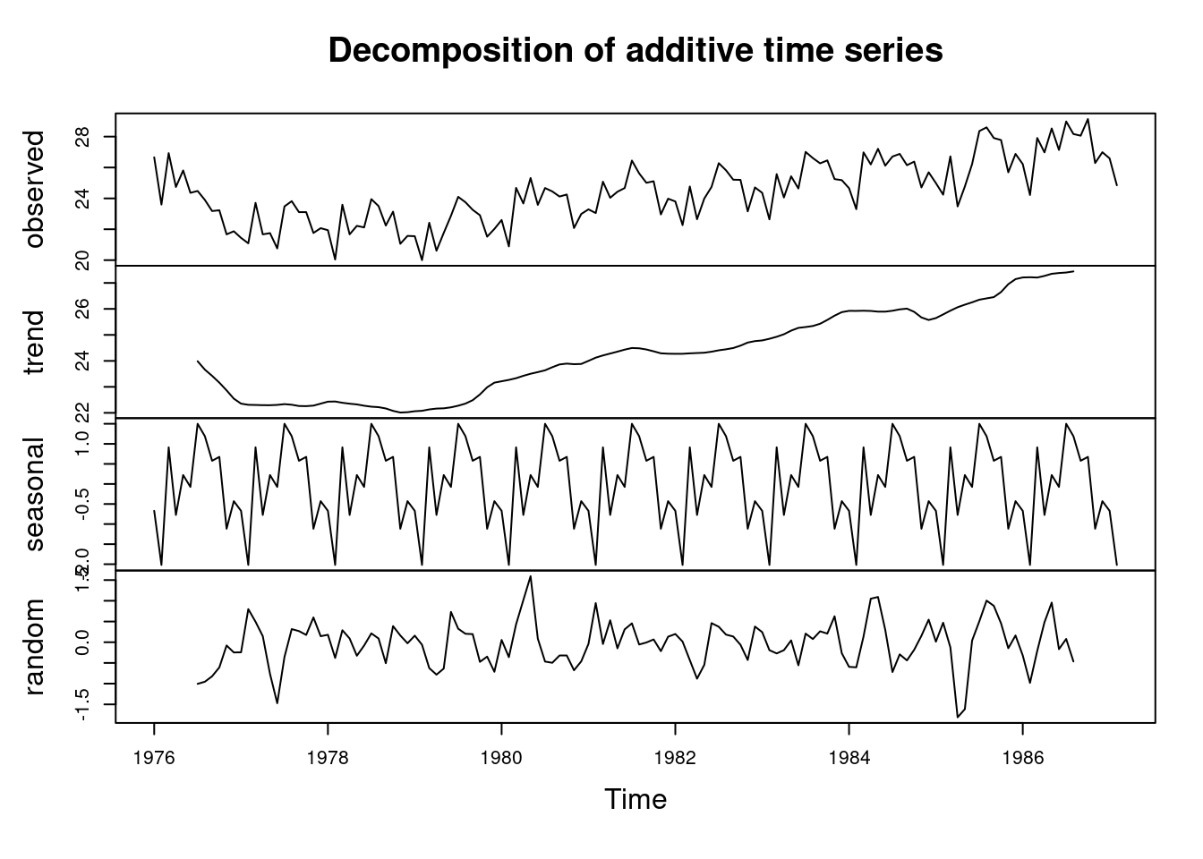
Models
Arima
I used an auto arima with a Box-Cox transformation. The model had for the the Non-seasonal part the following results: p = 0, d=1, q= 0, while for the seasonal part: p = 2, d=1, q= 2. In summary, first difference had to be applied to the variable and a relevant seasonal pattern was detected.
arima_model <- auto.arima(ts(train_df,frequency = 12,start = 1976), lambda='auto')
print(arima_model)
## Series: ts(train_df, frequency = 12, start = 1976)
## ARIMA(0,1,0)(2,1,1)[12]
## Box Cox transformation: lambda= 0.6710961
##
## Coefficients:
## sar1 sar2 sma1
## -0.4372 -0.2523 -0.7566
## s.e. 0.1371 0.1330 0.1711
##
## sigma^2 estimated as 0.04618: log likelihood=4.59
## AIC=-1.18 AICc=-0.83 BIC=10Drift model
The drift model was estimated with a Box-Cox transformation. Below I show the specification on this model.
##
## Forecast method: Random walk with drift
##
## Model Information:
## Call: rwf(y = ts(train_df, frequency = 12, start = 1976), h = length(test_df),
##
##  Call:     drift = TRUE, level = c(80, 95), fan = FALSE, lambda = "auto",
##
##  Call:     biasadj = TRUE, bootstrap = FALSE, npaths = 5000, x = train_df)
##
## Drift: -0.0351  (se 0.3279)
## Residual sd: 3.7821
##
## Error measures:
##               ME RMSE MAE MPE MAPE MASE ACF1
## Training set NaN  NaN NaN NaN  NaN  NaN   NA
##
## Forecasts:
##     Point Forecast    Lo 80    Hi 80      Lo 95    Hi 95
## 135       24.82334 22.91256 26.71743 21.8750943 27.69769
## 136       24.79646 22.07730 27.48177 20.5835450 28.85925
## 137       24.76935 21.41963 28.06759 19.5616767 29.74826
## 138       24.74203 20.85232 28.56210 18.6761833 30.49792
## 139       24.71449 20.34176 28.99891 17.8756320 31.15954
## 140       24.68673 19.87078 29.39515 17.1337141 31.75932
## 141       24.65874 19.42921 29.76099 16.4348183 32.31272
## 142       24.63053 19.01047 30.10300 15.7687649 32.82978
## 143       24.60210 18.60997 30.42572 15.1284596 33.31744
## 144       24.57344 18.22441 30.73245 14.5087040 33.78072
## 145       24.54456 17.85129 31.02567 13.9055328 34.22340
## 146       24.51546 17.48867 31.30730 13.3158176 34.64840
## 147       24.48613 17.13502 31.57884 12.7370165 35.05801
## 148       24.45657 16.78908 31.84152 12.1670079 35.45411
## 149       24.42679 16.44984 32.09635 11.6039749 35.83823
## 150       24.39678 16.11643 32.34416 11.0463219 36.21163
## 151       24.36654 15.78812 32.58565 10.4926125 36.57538
## 152       24.33607 15.46428 32.82142  9.9415191 36.93040
## 153       24.30537 15.14438 33.05198  9.3917810 37.27746
## 154       24.27445 14.82793 33.27777  8.8421675 37.61724
## 155       24.24329 14.51452 33.49919  8.2914403 37.95033
## 156       24.21191 14.20377 33.71658  7.7383153 38.27726
## 157       24.18029 13.89535 33.93022  7.1814166 38.59847
## 158       24.14844 13.58894 34.14040  6.6192202 38.91437
## 159       24.11635 13.28427 34.34735  6.0499767 39.22532
## 160       24.08404 12.98108 34.55128  5.4716017 39.53166
## 161       24.05149 12.67914 34.75239  4.8815051 39.83367
## 162       24.01870 12.37821 34.95084  4.2763124 40.13161
## 163       23.98568 12.07810 35.14680  3.6513664 40.42573
## 164       23.95243 11.77860 35.34041  2.9997411 40.71625
## 165       23.91893 11.47951 35.53180  2.3099795 41.00336
## 166       23.88520 11.18067 35.72110  1.5595211 41.28725
## 167       23.85124 10.88188 35.90840  0.6833618 41.56809
## 168       23.81703 10.58297 36.09381 -0.6229830 41.84602
Naive model
The naive model was estimated with a Box-Cox transformation. Below I show the specification on this model.
naive_model <- naive(ts(train_df,frequency = 12,start = 1976), level = c(80, 95), fan = FALSE, lambda = "auto",
                     biasadj = TRUE, bootstrap = FALSE, npaths = 5000, x = train_df, h = length(test_df) )
summary(naive_model)
##
## Forecast method: Naive method
##
## Model Information:
## Call: naive(y = ts(train_df, frequency = 12, start = 1976), h = length(test_df),
##
## Call: level = c(80, 95), fan = FALSE, lambda = "auto", biasadj = TRUE,
##
## Call: bootstrap = FALSE, npaths = 5000, x = train_df)
##
## Residual sd: 3.768
##
## Error measures:
## ME RMSE MAE MPE MAPE MASE ACF1
## Training set NaN NaN NaN NaN NaN NaN NA
##
## Forecasts:
## Point Forecast Lo 80 Hi 80 Lo 95 Hi 95
## 135 24.83720 22.93389 26.72396 21.900597 27.70052
## 136 24.82439 22.12656 27.48896 20.645047 28.85615
## 137 24.81159 21.50122 28.07177 19.666381 29.73381
## 138 24.79879 20.96989 28.56037 18.830186 30.46789
## 139 24.78598 20.49852 28.98884 18.084426 31.11038
## 140 24.77318 20.06963 29.37461 17.402417 31.68792
## 141 24.76038 19.67285 29.72807 16.768303 32.21633
## 142 24.74757 19.30144 30.05597 16.171745 32.70591
## 143 24.73477 18.95069 30.36299 15.605550 33.16379
## 144 24.72197 18.61720 30.65255 15.064469 33.59517
## 145 24.70916 18.29839 30.92722 14.544525 34.00399
## 146 24.69636 17.99224 31.18900 14.042617 34.39327
## 147 24.68356 17.69718 31.43948 13.556263 34.76544
## 148 24.67075 17.41190 31.67995 13.083435 35.12246
## 149 24.65795 17.13535 31.91148 12.622447 35.46594
## 150 24.64515 16.86663 32.13494 12.171871 35.79723
## 151 24.63234 16.60498 32.35109 11.730485 36.11747
## 152 24.61954 16.34977 32.56057 11.297220 36.42763
## 153 24.60674 16.10044 32.76393 10.871139 36.72856
## 154 24.59393 15.85651 32.96165 10.451401 37.02097
## 155 24.58113 15.61754 33.15416 10.037246 37.30552
## 156 24.56833 15.38317 33.34182 9.627980 37.58275
## 157 24.55552 15.15305 33.52497 9.222955 37.85318
## 158 24.54272 14.92689 33.70389 8.821563 38.11725
## 159 24.52992 14.70443 33.87886 8.423225 38.37536
## 160 24.51711 14.48542 34.05010 8.027378 38.62787
## 161 24.50431 14.26964 34.21784 7.633467 38.87509
## 162 24.49151 14.05689 34.38227 7.240938 39.11734
## 163 24.47870 13.84700 34.54356 6.849226 39.35487
## 164 24.46590 13.63978 34.70189 6.457743 39.58794
## 165 24.45310 13.43509 34.85739 6.065865 39.81676
## 166 24.44029 13.23279 35.01020 5.672920 40.04155
## 167 24.42749 13.03274 35.16046 5.278158 40.26249
## 168 24.41469 12.83482 35.30827 4.880733 40.47976Snaive model
The snaive model was estimated with a Box-Cox transformation. Below I show the specification on this model.
snaive_model <- snaive(ts(train_df,frequency = 12,start = 1976), level = c(80, 95), fan = FALSE,
       lambda = 'auto', biasadj = TRUE, bootstrap = FALSE, npaths = 5000,
       x = train_df, h = length(test_df) )
summary(snaive_model)
##
## Forecast method: Seasonal naive method
##
## Model Information:
## Call: snaive(y = ts(train_df, frequency = 12, start = 1976), h = length(test_df),
##
## Call: level = c(80, 95), fan = FALSE, lambda = "auto", biasadj = TRUE,
##
## Call: bootstrap = FALSE, npaths = 5000, x = train_df)
##
## Residual sd: 3.768
##
## Error measures:
## ME RMSE MAE MPE MAPE MASE ACF1
## Training set NaN NaN NaN NaN NaN NaN NA
##
## Forecasts:
## Point Forecast Lo 80 Hi 80 Lo 95 Hi 95
## 135 24.83720 22.93389 26.72396 21.900597 27.70052
## 136 24.82439 22.12656 27.48896 20.645047 28.85615
## 137 24.81159 21.50122 28.07177 19.666381 29.73381
## 138 24.79879 20.96989 28.56037 18.830186 30.46789
## 139 24.78598 20.49852 28.98884 18.084426 31.11038
## 140 24.77318 20.06963 29.37461 17.402417 31.68792
## 141 24.76038 19.67285 29.72807 16.768303 32.21633
## 142 24.74757 19.30144 30.05597 16.171745 32.70591
## 143 24.73477 18.95069 30.36299 15.605550 33.16379
## 144 24.72197 18.61720 30.65255 15.064469 33.59517
## 145 24.70916 18.29839 30.92722 14.544525 34.00399
## 146 24.69636 17.99224 31.18900 14.042617 34.39327
## 147 24.68356 17.69718 31.43948 13.556263 34.76544
## 148 24.67075 17.41190 31.67995 13.083435 35.12246
## 149 24.65795 17.13535 31.91148 12.622447 35.46594
## 150 24.64515 16.86663 32.13494 12.171871 35.79723
## 151 24.63234 16.60498 32.35109 11.730485 36.11747
## 152 24.61954 16.34977 32.56057 11.297220 36.42763
## 153 24.60674 16.10044 32.76393 10.871139 36.72856
## 154 24.59393 15.85651 32.96165 10.451401 37.02097
## 155 24.58113 15.61754 33.15416 10.037246 37.30552
## 156 24.56833 15.38317 33.34182 9.627980 37.58275
## 157 24.55552 15.15305 33.52497 9.222955 37.85318
## 158 24.54272 14.92689 33.70389 8.821563 38.11725
## 159 24.52992 14.70443 33.87886 8.423225 38.37536
## 160 24.51711 14.48542 34.05010 8.027378 38.62787
## 161 24.50431 14.26964 34.21784 7.633467 38.87509
## 162 24.49151 14.05689 34.38227 7.240938 39.11734
## 163 24.47870 13.84700 34.54356 6.849226 39.35487
## 164 24.46590 13.63978 34.70189 6.457743 39.58794
## 165 24.45310 13.43509 34.85739 6.065865 39.81676
## 166 24.44029 13.23279 35.01020 5.672920 40.04155
## 167 24.42749 13.03274 35.16046 5.278158 40.26249
## 168 24.41469 12.83482 35.30827 4.880733 40.47976Stl model
Below I show the specification on this model.
stl_model <- stl(ts(train_df,frequency = 12,start = 1976), s.window = 12, t.window = 12, t.jump = 1)
summary(stl_model)
## Call:
## stl(x = ts(train_df, frequency = 12, start = 1976), s.window = 12,
## t.window = 12, t.jump = 1)
##
## Time.series components:
## seasonal trend remainder
## Min. :-2.1696016 Min. :21.90544 Min. :-1.4192859
## 1st Qu.:-0.6866532 1st Qu.:22.59791 1st Qu.:-0.2434104
## Median :-0.0220175 Median :24.40128 Median : 0.0203580
## Mean :-0.0179313 Mean :24.44334 Mean :-0.0091438
## 3rd Qu.: 0.8119665 3rd Qu.:25.78991 3rd Qu.: 0.2328295
## Max. : 1.5454074 Max. :27.53841 Max. : 1.3195528
## IQR:
## STL.seasonal STL.trend STL.remainder data
## 1.4986 3.1920 0.4762 3.1375
## % 47.8 101.7 15.2 100.0
##
## Weights: all == 1
##
## Other components: List of 5
## $ win : Named num [1:3] 12 12 13
## $ deg : Named int [1:3] 0 1 1
## $ jump : Named num [1:3] 2 1 2
## $ inner: int 2
## $ outer: int 0Holt-Winters (additive & multiplicative)
The hw additive & multiplicative models was estimated with a Box-Cox transformation. Below I show the specification on this model. Moreover, they used a damped trend.
hw_additive <- hw(ts(train_df,frequency = 12,start = 1976) ,
                  seasonal="additive", m= 12, lambda="auto", damped= TRUE, h=length(test_df))
cat('additive model summary\n')
## additive model summarysummary(hw_additive)##
## Forecast method: Damped Holt-Winters' additive method
##
## Model Information:
## Damped Holt-Winters' additive method
##
## Call:
## hw(y = ts(train_df, frequency = 12, start = 1976), h = length(test_df),
##
## Call:
## seasonal = "additive", damped = TRUE, lambda = "auto", m = 12)
##
## Box-Cox transformation: lambda= 0.6711
##
## Smoothing parameters:
## alpha = 0.8278
## beta = 2e-04
## gamma = 0.0075
## phi = 0.9098
##
## Initial states:
## l = 12.3481
## b = -0.2367
## s = -0.1088 -0.3909 0.2734 0.211 0.3974 0.4549
## -0.0421 0.0671 -0.2706 0.331 -0.7103 -0.2121
##
## sigma: 0.2168
##
## AIC AICc BIC
## 264.4321 270.3799 316.5932
##
## Error measures:
## ME RMSE MAE MPE MAPE MASE
## Training set 0.05520405 0.5791917 0.4503309 0.1990123 1.842102 0.4544282
## ACF1
## Training set 0.05843258
##
## Forecasts:
## Point Forecast Lo 80 Hi 80 Lo 95 Hi 95
## Mar 1987 27.96634 27.13937 28.80142 26.70492 29.24675
## Apr 1987 26.18557 25.13679 27.24834 24.58734 27.81654
## May 1987 27.18369 25.92567 28.46115 25.26770 29.14517
## Jun 1987 26.85080 25.42976 28.29702 24.68786 29.07265
## Jul 1987 28.34337 26.74367 29.97335 25.90929 30.84826
## Aug 1987 28.15025 26.41552 29.92088 25.51201 30.87247
## Sep 1987 27.59537 25.74497 29.48753 24.78266 30.50575
## Oct 1987 27.78772 25.81390 29.80877 24.78856 30.89739
## Nov 1987 25.83006 23.79502 27.91928 22.74018 29.04668
## Dec 1987 26.64753 24.48632 28.86801 23.36683 30.06690
## Jan 1988 26.35591 24.10351 28.67350 22.93824 29.92610
## Feb 1988 24.90024 22.59782 27.27494 21.40907 28.56052
## Mar 1988 27.96621 25.47670 30.53087 24.19008 31.91817
## Apr 1988 26.18546 23.66360 28.78988 22.36302 30.20110
## May 1988 27.18359 24.54406 29.91027 23.18311 31.38801
## Jun 1988 26.85071 24.14000 29.65461 22.74393 31.17555
## Jul 1988 28.34329 25.50097 31.28265 24.03682 32.87683
## Aug 1988 28.15017 25.23580 31.16738 23.73598 32.80501
## Sep 1988 27.59530 24.62472 30.67505 23.09783 32.34822
## Oct 1988 27.78765 24.73588 30.95393 23.16829 32.67497
## Nov 1988 25.83001 22.78316 29.00001 21.22192 30.72630
## Dec 1988 26.64748 23.49843 29.92406 21.88493 31.70848
## Jan 1989 26.35586 23.15103 29.69441 21.51067 31.51400
## Feb 1989 24.90020 21.69252 28.25004 20.05433 30.07880
## Mar 1989 27.96617 24.56058 31.51408 22.81755 33.44785
## Apr 1989 26.18542 22.79270 29.72941 21.06042 31.66449
## May 1989 27.18356 23.68401 30.83809 21.89672 32.83316
## Jun 1989 26.85068 23.30454 30.55814 21.49532 32.58363
## Jul 1989 28.34326 24.66896 32.18148 22.79294 34.27725
## Aug 1989 28.15015 24.42424 32.04594 22.52348 34.17446
## Sep 1989 27.59528 23.83607 31.53116 21.92063 33.68347
## Oct 1989 27.78763 23.96143 31.79569 22.01275 33.98820
## Nov 1989 25.82999 22.04370 29.80850 20.12077 31.98921
## Dec 1989 26.64746 22.76480 30.72599 20.79236 32.96108hw_multiplicative <- hw(ts(train_df,frequency = 12,start = 1976),
seasonal="multiplicative", m= 12, lambda=NULL, damped= TRUE,h=length(test_df))
cat('multiplicative model summary\n')## multiplicative model summarysummary(hw_multiplicative)##
## Forecast method: Damped Holt-Winters' multiplicative method
##
## Model Information:
## Damped Holt-Winters' multiplicative method
##
## Call:
## hw(y = ts(train_df, frequency = 12, start = 1976), h = length(test_df),
##
## Call:
## seasonal = "multiplicative", damped = TRUE, lambda = NULL,
##
## Call:
## m = 12)
##
## Smoothing parameters:
## alpha = 0.7541
## beta = 0.0087
## gamma = 1e-04
## phi = 0.9675
##
## Initial states:
## l = 25.5802
## b = -0.2795
## s = 0.9832 0.9532 1.0286 1.0205 1.0446 1.0573
## 0.9978 1.0129 0.9686 1.0385 0.9153 0.9795
##
## sigma: 0.027
##
## AIC AICc BIC
## 560.6326 566.5804 612.7937
##
## Error measures:
## ME RMSE MAE MPE MAPE MASE
## Training set 0.07476038 0.6071546 0.4533434 0.2795672 1.84821 0.4574681
## ACF1
## Training set 0.1146113
##
## Forecasts:
## Point Forecast Lo 80 Hi 80 Lo 95 Hi 95
## Mar 1987 28.22983 27.25318 29.20648 26.73617 29.72349
## Apr 1987 26.33558 25.18961 27.48154 24.58297 28.08818
## May 1987 27.54943 26.14322 28.95564 25.39882 29.70004
## Jun 1987 27.14538 25.57837 28.71240 24.74884 29.54193
## Jul 1987 28.77026 26.93389 30.60663 25.96177 31.57874
## Aug 1987 28.43224 26.45620 30.40829 25.41014 31.45435
## Sep 1987 27.78380 25.70455 29.86305 24.60386 30.96374
## Oct 1987 28.01173 25.77349 30.24998 24.58863 31.43484
## Nov 1987 25.96344 23.76309 28.16378 22.59830 29.32857
## Dec 1987 26.78599 24.39123 29.18074 23.12352 30.44845
## Jan 1988 26.69138 24.18515 29.19762 22.85843 30.52434
## Feb 1988 24.94746 22.49640 27.39852 21.19889 28.69603
## Mar 1988 28.31180 25.41048 31.21311 23.87462 32.74898
## Apr 1988 26.40953 23.59446 29.22461 22.10424 30.71483
## May 1988 27.62426 24.56876 30.67976 22.95128 32.29724
## Jun 1988 27.21669 24.09945 30.33394 22.44928 31.98411
## Jul 1988 28.84336 25.42898 32.25774 23.62152 34.06520
## Aug 1988 28.50212 25.02080 31.98344 23.17790 33.82634
## Sep 1988 27.84984 24.34527 31.35442 22.49006 33.20963
## Oct 1988 28.07614 24.44116 31.71111 22.51692 33.63535
## Nov 1988 26.02117 22.55937 29.48297 20.72681 31.31554
## Dec 1988 26.84360 23.17811 30.50909 21.23772 32.44949
## Jan 1989 26.74691 23.00212 30.49171 21.01975 32.47408
## Feb 1989 24.99766 21.41259 28.58273 19.51477 30.48055
## Mar 1989 28.36691 24.20330 32.53052 21.99921 34.73460
## Apr 1989 26.45926 22.48794 30.43057 20.38566 32.53285
## May 1989 27.67457 23.43031 31.91882 21.18354 34.16559
## Jun 1989 27.26464 22.99518 31.53409 20.73507 33.79420
## Jul 1989 28.89250 24.27595 33.50906 21.83209 35.95292
## Aug 1989 28.54910 23.89739 33.20080 21.43492 35.66327
## Sep 1989 27.89424 23.26229 32.52620 20.81028 34.97821
## Oct 1989 28.11943 23.36341 32.87545 20.84573 35.39314
## Nov 1989 26.05999 21.57284 30.54714 19.19749 32.92249
## Dec 1989 26.88233 22.17250 31.59217 19.67926 34.08541Predictions of test data
Then, I saved the predictions of the test data for each model.
pred_arima <- forecast(arima_model, h = length(test_df))
pred_drift <- drift_model
pred_naive <- naive_model
pred_snaive <- snaive_model
pred_stl <- forecast(stl_model,h= length(test_df))
pred_hw_add <- hw_additive
pred_hw_mult <- hw_multiplicative
Compare results of each models
Here, I made a graph in order to compare the models performance.
arima_compare = create_df_compare(test_df, c(pred_arima$mean))
drift_compare = create_df_compare(test_df, c(pred_drift$mean))
naive_compare = create_df_compare(test_df, c(pred_naive$mean))
snaive_compare = create_df_compare(test_df, c(pred_snaive$mean))
stl_compare = create_df_compare(test_df, c(pred_stl$mean))
hw_add_compare = create_df_compare(test_df, c(pred_hw_add$mean))
hw_mult_compare = create_df_compare(test_df, c(pred_hw_mult$mean))

plot_df(arima_compare, "Results Real vs Arima" )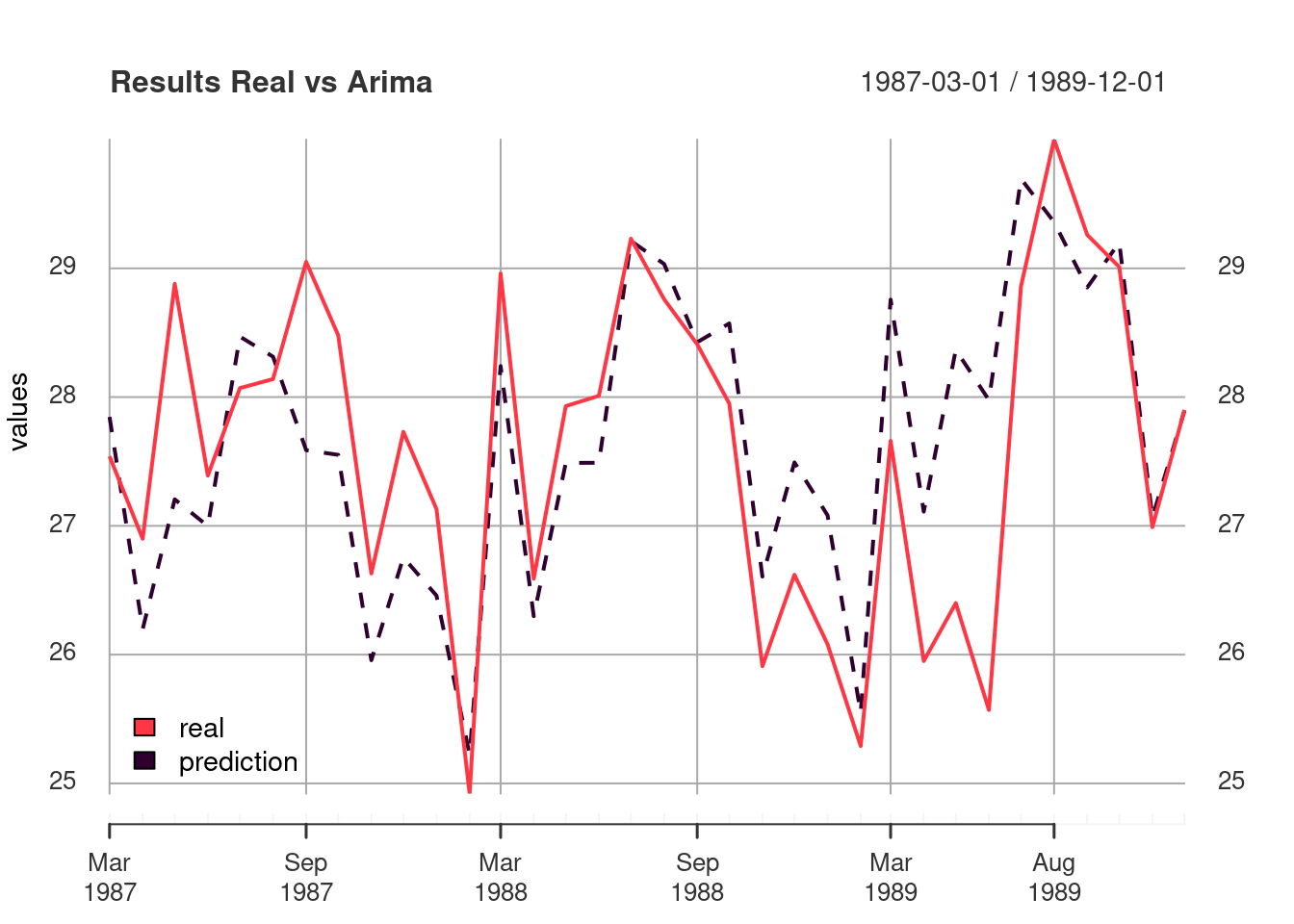
plot_df(drift_compare, "Results Real vs drift" )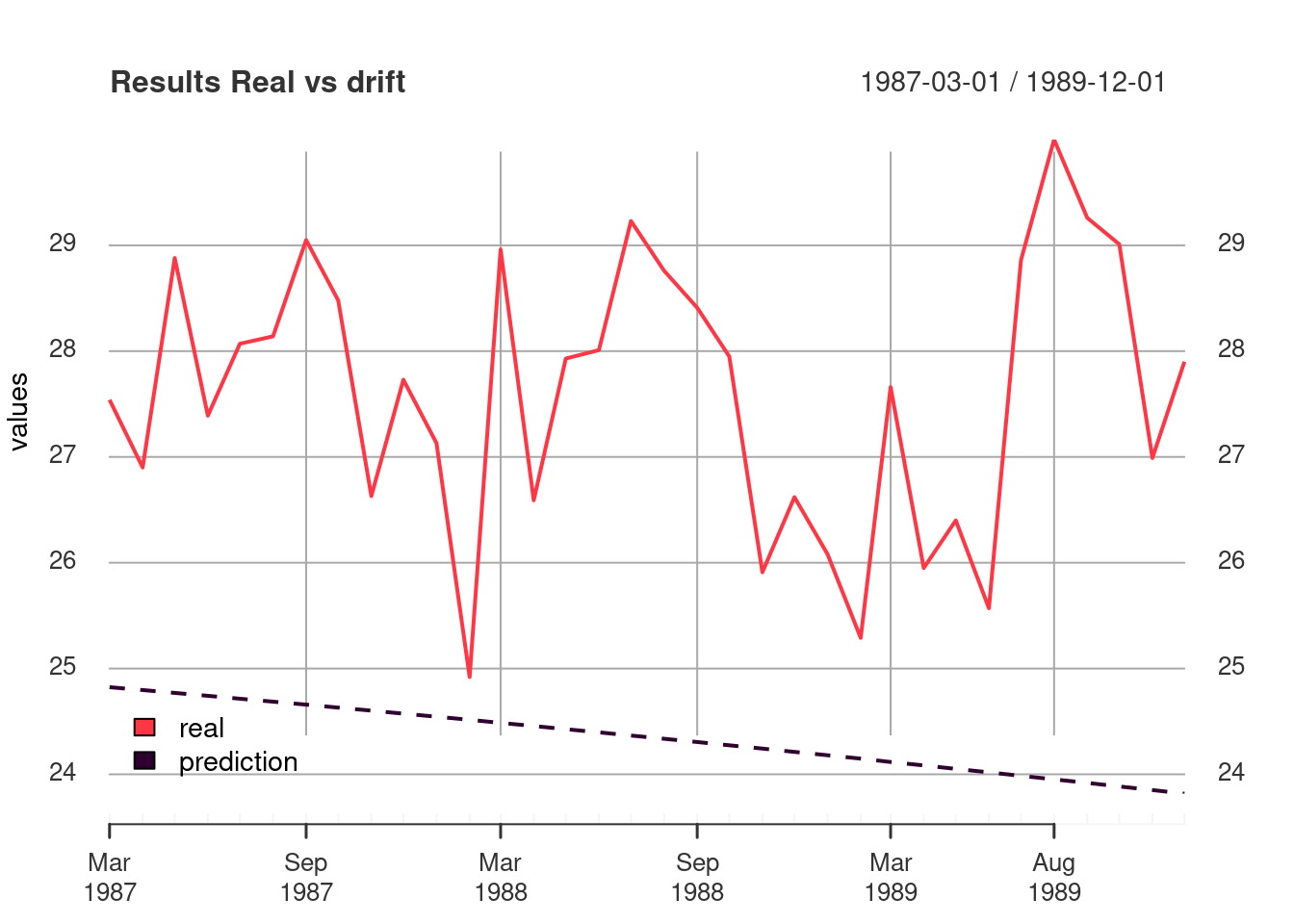
plot_df(naive_compare, "Results Real vs Naive" )
plot_df(snaive_compare, "Results Real vs Snaive" )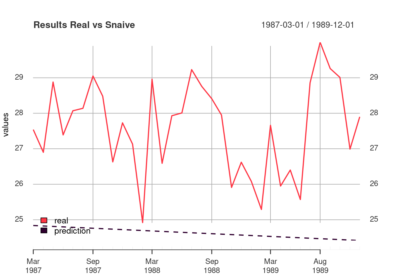
plot_df(stl_compare, "Results Real vs Stl" )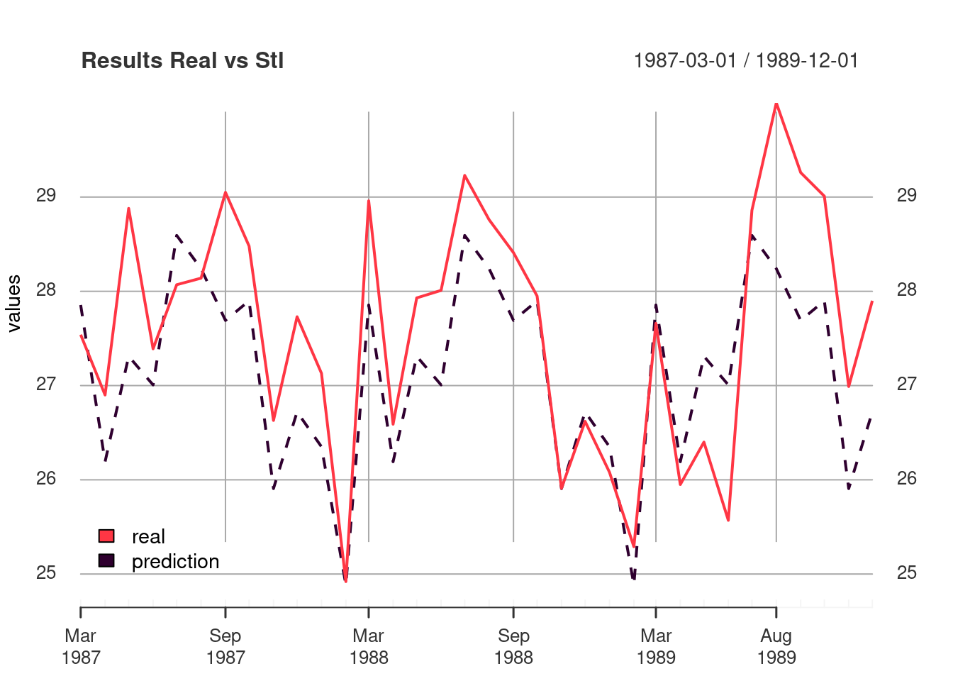
plot_df(hw_add_compare, "Results Real vs Hw. Add." )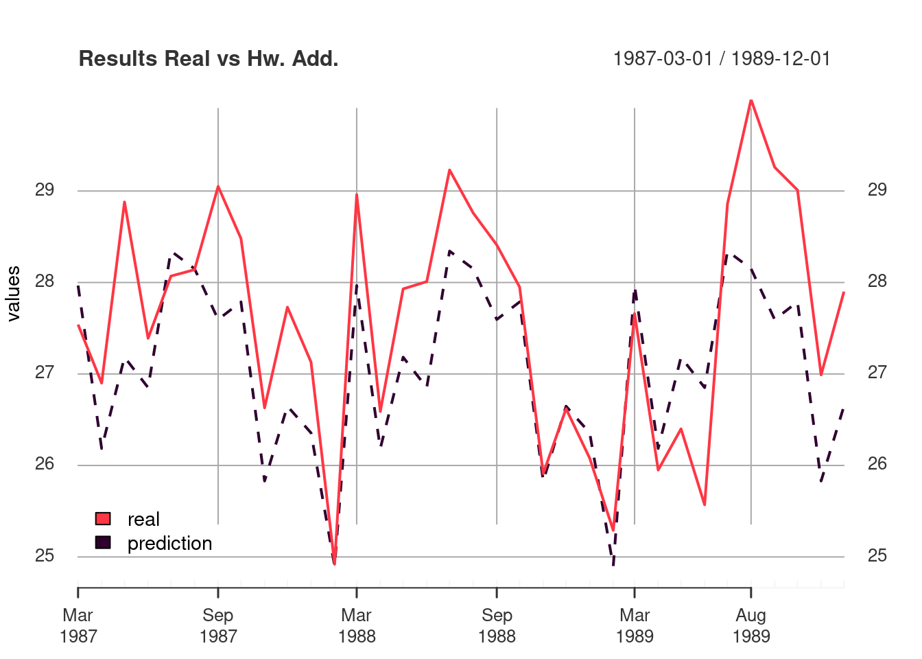
plot_df(hw_mult_compare, "Results Real vs Hw. Mult." )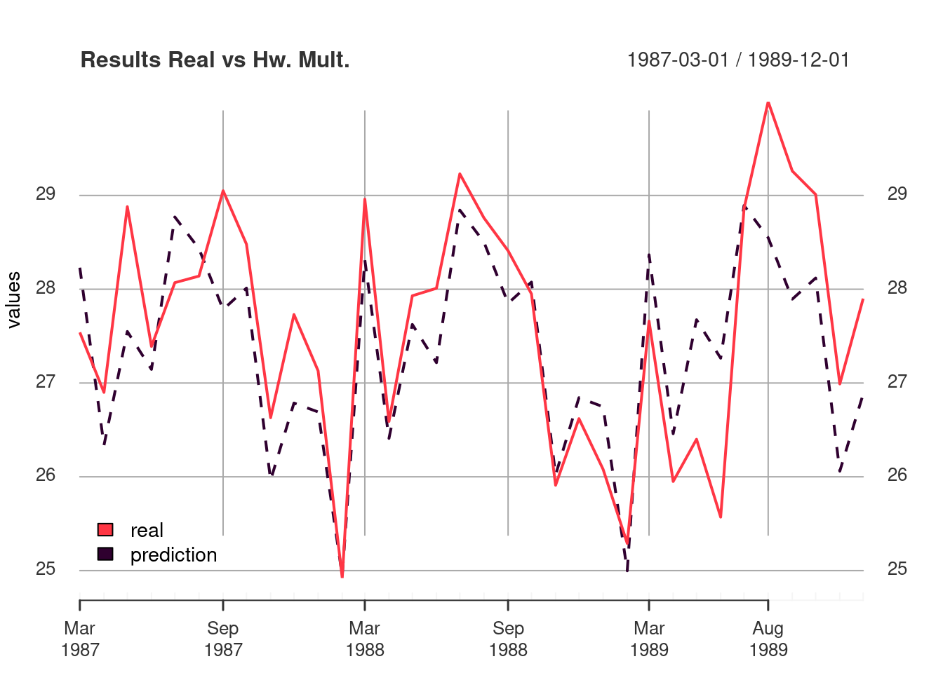
RMSE for each model
Now, I compute the rmse using the test data and the predictions of each model.
rmse_arima <- rmse( c(pred_arima$mean),test_df )
rmse_drift <- rmse(  c(pred_drift$mean), test_df )
rmse_naive <- rmse(  c(pred_naive$mean), test_df )
rmse_snaive <- rmse(  c(pred_snaive$mean), test_df )
rmse_stl <- rmse(  c(pred_stl$mean), test_df )
rmse_hw_add <- rmse(  c(pred_hw_add$mean), test_df )
rmse_hw_mult <- rmse(  c(pred_hw_mult$mean), test_df )
Results
I saved the results in a data frame sorted by rmse in ascending order where the first row is the best model with the lowest rmse. The best model was hw multiplicative with a rmse of 0.78 and the worst was drift model with a rmse of 3.49.
df_rmse <- data.frame(method= c('arima', 'drift', 'naive', 'snaive', 'stl', 'hw_additive', 'hw_multiplicative'),
              rmse_values = c(rmse_arima, rmse_drift, rmse_naive, rmse_snaive, rmse_stl, rmse_hw_add, rmse_hw_mult) ) %>%
  arrange((rmse_values))

df_rmse
## method rmse_values
## 1 hw_multiplicative 0.7818894
## 2 stl 0.8481321
## 3 arima 0.8754021
## 4 hw_additive 0.8968844
## 5 naive 3.2261873
## 6 snaive 3.2261873
## 7 drift 3.4999880Alex Amaguaya
Research Assistant / Data Scientist
My research interests are Networks and the intersection between Econometrics and Machine Learning.