Exploratory Data Analysis

The average income of the Control Group is more bigger than the Treatment Group in 1974 (5619 vs 2095)

table_comp_74 <-lalonde %>% 
  group_by(treat) %>% 
  summarise_at( vars(re74), list(mean = mean, median = median ))
head(table_comp_74)
## # A tibble: 2 × 3
##   treat  mean median
##   <int> <dbl>  <dbl>
## 1     0 5619.  2547.
## 2     1 2096.     0

The difference in mean income of the Control and Treatment groups appear to be reduced in 1978. (6984 vs 6349)

table_comp_78 <-lalonde %>% 
  group_by(treat) %>% 
  summarise_at( vars(re78), list(mean = mean, median = median ))
head(table_comp_78)
## # A tibble: 2 × 3
##   treat  mean median
##   <int> <dbl>  <dbl>
## 1     0 6984.  4976.
## 2     1 6349.  4232.

The control group has higher earning that the treatment group - does this mean the treatment had a negative impact?

library(scales)
par(mfrow=c(3,1), mar=c(3,4,3,1))
lalonde %>% 
  filter( treat ==1 ) %>%
  with(hist(re74 ,col='skyblue',border=FALSE,breaks= 20,
            main='Earning distribution of treatment and control 74')) 
lalonde %>% 
  filter( treat ==0 ) %>%
  with(hist(re74 ,col=scales::alpha('red',.5),breaks= 20, border=FALSE, add=TRUE,
            main='Earning distribution of treatment and control 74'))
legend(x=30000,y=100,c("treatment","control"),cex=.8,col=c("skyblue",scales::alpha('red',.5)),
       fill=c("skyblue",scales::alpha('red',.5)))

lalonde %>% 
  filter( treat ==1 ) %>%
  with(hist(educ ,col='skyblue',border=FALSE,breaks= 20,
            main='Educ. distribution of treatment and control')) 
lalonde %>% 
  filter( treat ==0 ) %>%
  with(hist(educ ,col=scales::alpha('red',.5),breaks= 20, border=FALSE, add=TRUE,
            main='Edu. of treatment and control'))
legend(x=14,y=40,c("treatment","control"),cex=.8,col=c("skyblue",scales::alpha('red',.5)),
       fill=c("skyblue",scales::alpha('red',.5)))

lalonde %>% 
  filter( treat ==1 ) %>%
  with(hist(age ,col='skyblue',border=FALSE,breaks= 20,
            main='Age distribution of treatment and control')) 
lalonde %>% 
  filter( treat ==0 ) %>%
  with(hist(age ,col=scales::alpha('red',.5),breaks= 20, border=FALSE, add=TRUE,
            main='Age of treatment and control'))
legend(x=45,y=24,c("treatment","control"),cex=.8,col=c("skyblue",scales::alpha('red',.5)),
       fill=c("skyblue",scales::alpha('red',.5)))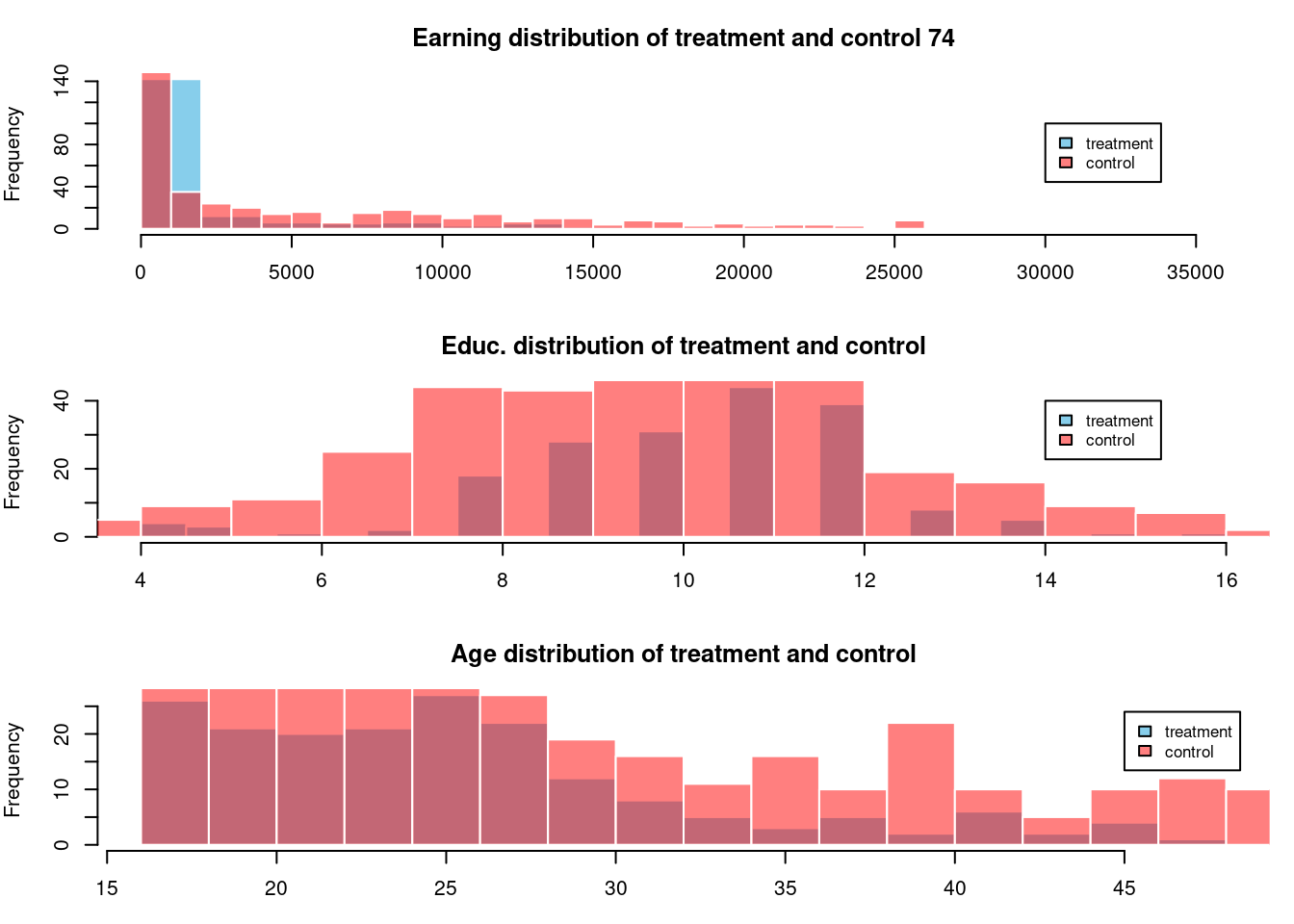

Matching Process

After processing data, I run an logit model to analysis some previous results about Propensity score model. It used the treatment variable like depend variable and the others variables are independent variables. The equation looks something like this:

\[P\left(treatment_{i}=1|X\right) = age_{i}+edu_{i}+married_{i}+nodegree_{i}+re78_{i}+black_{i}+hispan_{i}\]

I estimate that equation and analyze the beta coefficients and their statistical significant. Also, the white dummy variable is omitted when I estimate the equation.

The results show:

• educ, nodegree, black, hispan have a positive relationship with the treatment variable and are statistically significant.
• married has a negative relationship with the treatment variable and is statistically significant.

library(glm2)
propensity.score.model <- glm(treat ~ age+educ+married+nodegree+black+hispan,family=binomial() , data= lalonde)
pscore <- propensity.score.model$fitted.values
summary(propensity.score.model)
## 
## Call:
## glm(formula = treat ~ age + educ + married + nodegree + black + 
##     hispan, family = binomial(), data = lalonde)
## 
## Deviance Residuals: 
##     Min       1Q   Median       3Q      Max  
## -1.7709  -0.4606  -0.2963   0.7766   2.6384  
## 
## Coefficients:
##             Estimate Std. Error z value Pr(>|z|)    
## (Intercept) -4.67874    1.02120  -4.582 4.61e-06 ***
## age          0.01030    0.01329   0.775  0.43857    
## educ         0.15161    0.06568   2.308  0.02098 *  
## married     -0.92969    0.27128  -3.427  0.00061 ***
## nodegree     0.78719    0.33507   2.349  0.01881 *  
## black        3.12657    0.28514  10.965  < 2e-16 ***
## hispan       0.99947    0.42191   2.369  0.01784 *  
## ---
## Signif. codes:  0 '***' 0.001 '**' 0.01 '*' 0.05 '.' 0.1 ' ' 1
## 
## (Dispersion parameter for binomial family taken to be 1)
## 
##     Null deviance: 751.49  on 613  degrees of freedom
## Residual deviance: 494.70  on 607  degrees of freedom
## AIC: 508.7
## 
## Number of Fisher Scoring iterations: 5

After analyzing the results, I apply the matching method to form the new control and treatment groups. The following shows the parameters used by the function:

matchit(formula, data, method = "nearest", distance = "logit",
               distance.options = list(), discard = "none",
               reestimate = FALSE, ...)

Where: These are the main arguments:

• formula: this argument takes the usual syntax of R formula.
• data: this argument specifies the used data.
• method: this argument specifies a matching method.
  • “exact” (exact matching)
  • “full” (full matching)
  • “genetic” (genetic matching)
  • “nearest” (nearest neighbor matching), it’s the default option.
  • “optimal” (optimal matching)
  • “subclass” (subclassification)
• distance: this argument specifies the method used to estimate the distance measure (logistic regression “logit” is the default option).
• discard: this argument specifies whether to discard units that fall outside some measure of support of the distance score before matching, and not allow them to be used at all in the matching procedure. Note that discarding units may change the quantity of interest being estimated. The options are:
  • “none” is the default, which discards no units before matching
  • “both” which discards all units (treated and control) that are outside the support of the distance measure
  • “control” which discards only control units outside the support of the distance measure of the treated units
  • “treat” which discards only treated units outside the support of the distance measure of the control units.
• reestimate: this argument specifies whether the model for distance measure should be re-estimated after units are discarded. The input must be a logical value. The default is FALSE.
• ratio: it’s about how many control units should be matched to each treated unit in k:1 matching.

Here, I apply the matchit process with a ratio of 2.

match_method <- matchit(treat ~ age+educ+married+nodegree+black+hispan , 
                        data=lalonde,  method='nearest',ratio= 2 )
match_method
## A matchit object
##  - method: Variable ratio 2:1 nearest neighbor matching without replacement
##  - distance: Propensity score
##              - estimated with logistic regression
##  - number of obs.: 614 (original), 555 (matched)
##  - target estimand: ATT
##  - covariates: age, educ, married, nodegree, black, hispan

Then, I show the propensity score distribution before and after matching. You can see that there are many observations with a probability or propensity score less than 0.15.

plot(match_method ,type='jitter')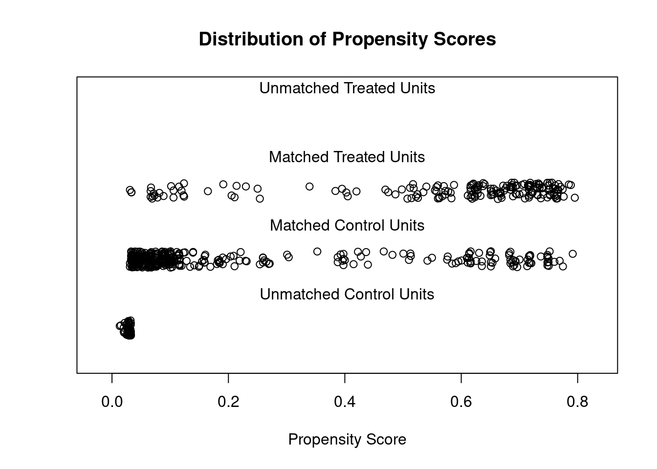

## [1] "To identify the units, use first mouse button; to stop, use second."
## integer(0)

A histogram plot is shown below and you can see that the propensity score distribution for the treated and control groups doesn’t change significantly (before & after Matching)

plot(match_method, type='hist', col.axis=4 )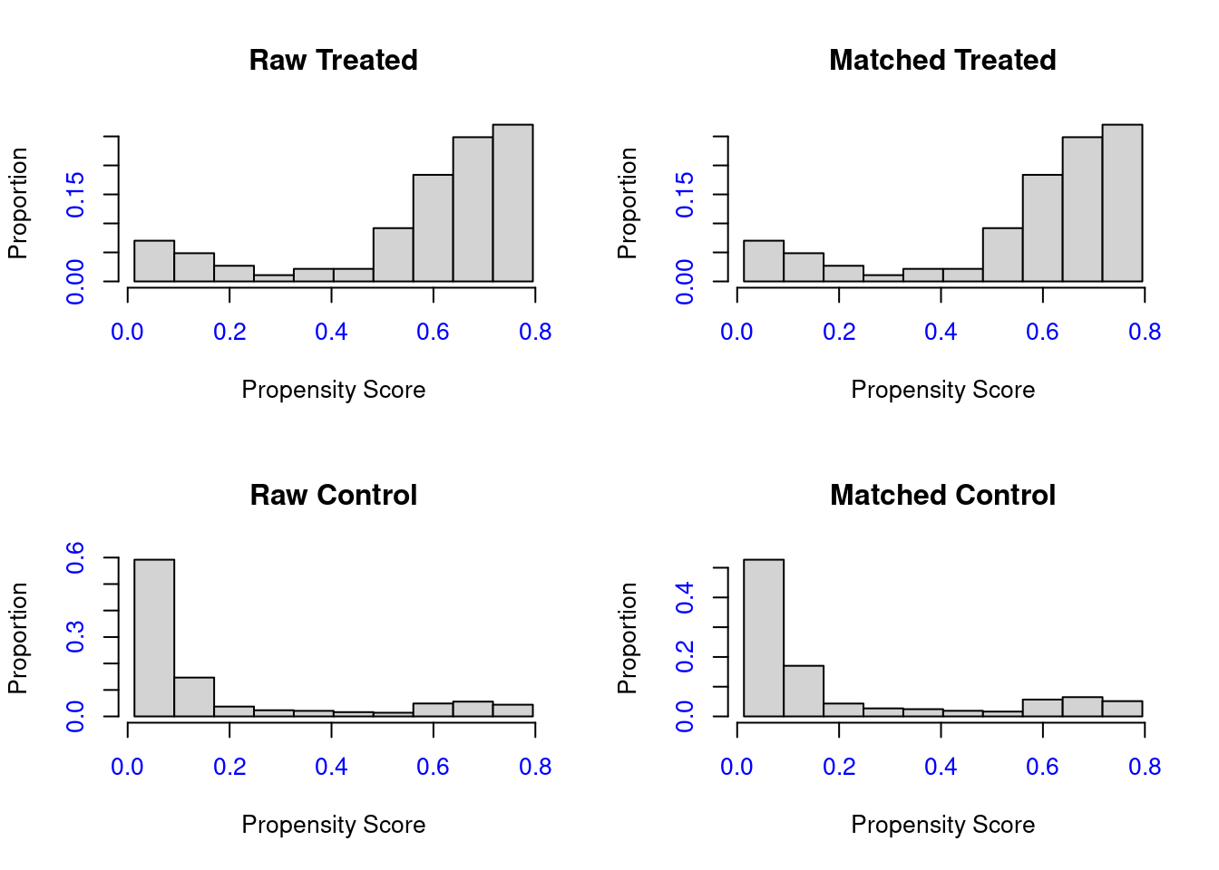

Mean difference of each variable for before and after match process

library(cobalt)
love.plot(bal.tab(match_method,binary='std', m.threshold=0.3),
          stat='mean.diffs', abs=F, shapes=c('triangle filled', 'circle filled'),
          colors = c("red", "blue"), sample.names = c("Before Match", "After Match") )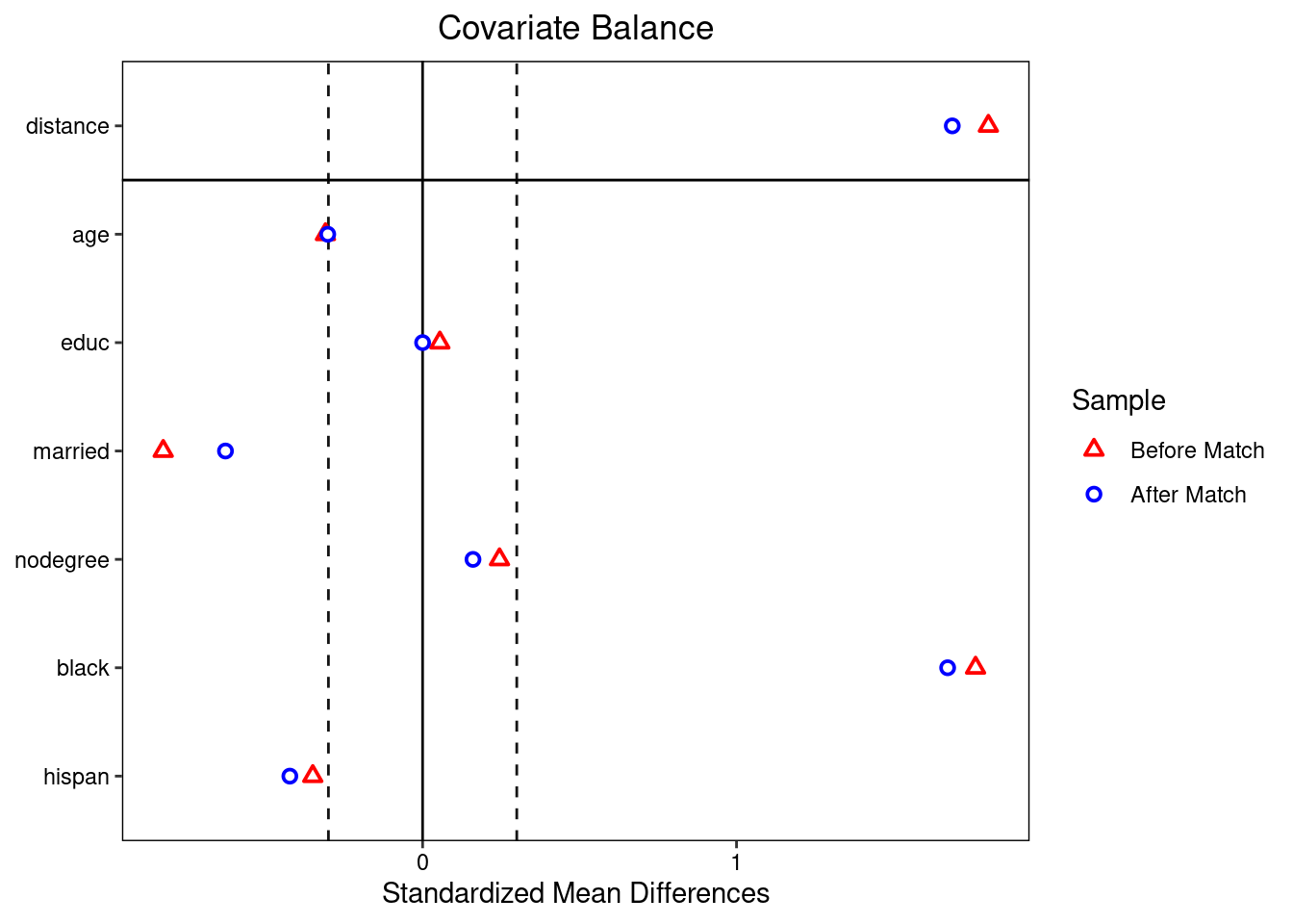

Now, I save the new treatment and control groups and can used for estimate model.

new_treat <- match.data(match_method, group='treat')
new_control <- match.data(match_method, group='control')